Bradford

This work is based on data from OpenPrescribing.

Obtaining boundaries

library(sf)

Linking to GEOS 3.13.0, GDAL 3.10.1, PROJ 9.5.1; sf_use_s2() is TRUE

library(tidyverse)

── Attaching core tidyverse packages ──────────────────────── tidyverse 2.0.0 ──
✔ dplyr     1.1.4     ✔ readr     2.1.5
✔ forcats   1.0.0     ✔ stringr   1.5.1
✔ ggplot2   3.5.1     ✔ tibble    3.2.1
✔ lubridate 1.9.4     ✔ tidyr     1.3.1
✔ purrr     1.0.4     

── Conflicts ────────────────────────────────────────── tidyverse_conflicts() ──
✖ dplyr::filter() masks stats::filter()
✖ dplyr::lag()    masks stats::lag()
ℹ Use the conflicted package (<http://conflicted.r-lib.org/>) to force all conflicts to become errors

library(tmap)
library(OpenStreetMap)

NHS boundaries

CCG_boundaries <- geojsonsf::geojson_sf("https://openprescribing.net/api/1.0/org_location/?org_type=ccg") |> st_transform(27700)

Warning in readLines(con): incomplete final line found on
'https://openprescribing.net/api/1.0/org_location/?org_type=ccg'

GP surgeries

Approximate locations of all registered GP surgeries can be obtained. For example, for Bradford (ICB code: 36J)

bradford_code <- "36J"

Reading the built-up areas data

builtup_bounds <- st_read("OS Open Built Up Areas.gpkg",
                          layer = "os_open_built_up_areas")

Reading layer `os_open_built_up_areas' from data source 
  `C:\Users\ts18jpf\OneDrive - University of Leeds\03_PhD\00_Misc_projects\Eng-Presc-Data\OS Open Built Up Areas.gpkg' 
  using driver `GPKG'
Simple feature collection with 8585 features and 7 fields
Geometry type: MULTIPOLYGON
Dimension:     XY
Bounding box:  xmin: 65300 ymin: 10000 xmax: 655625 ymax: 1177650
Projected CRS: OSGB36 / British National Grid

Selecting the biggest builtup area within the NHS region

bradford_zones <- builtup_bounds[CCG_boundaries[CCG_boundaries$code==bradford_code,],] |> slice_max(geometry_area_m)

Bradford_Practices <- geojsonsf::geojson_sf(
  paste0("https://openprescribing.net/api/1.0/org_location/?q=",
         bradford_code)
  ) |> st_transform(27700)

Warning in readLines(con): incomplete final line found on
'https://openprescribing.net/api/1.0/org_location/?q=36J'

tmap_mode("view")

ℹ tmap mode set to "view".

qtm(Bradford_Practices |> st_make_valid())

Short acting beta agonist inhalers

See: https://openprescribing.net/measure/saba/definition/

Taken from the web:

Why it matters: Why Asthma Still Kills reports that high use of short acting beta agonists (salbutamol and terbutaline) and poor adherence to inhaled corticosteroids in asthma suggests poor control - these patients should be reviewed regularly to ensure good control.

The NHS England National Medicines Optimisation Opportunities for 2023/24 identify improving patient outcomes from the use of inhalers as an area for improvement.

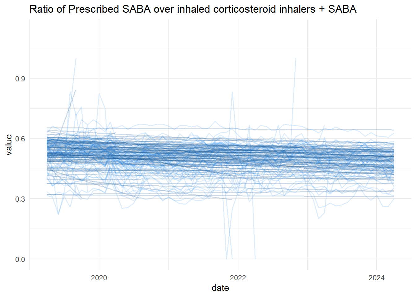
Description: Prescribing of short acting beta agonist (SABA) inhalers - salbutamol and terbutaline - compared with prescribing of inhaled corticosteroid inhalers and SABA inhalers

saba <- read_csv(
  paste0("https://openprescribing.net/api/1.0/measure_by_practice/?format=csv&org=",
         bradford_code,
         "&parent_org_type=ccg&measure=saba")) 

Rows: 5368 Columns: 9
── Column specification ────────────────────────────────────────────────────────
Delimiter: ","
chr  (4): measure, org_type, org_id, org_name
dbl  (4): numerator, denominator, calc_value, percentile
date (1): date

ℹ Use `spec()` to retrieve the full column specification for this data.
ℹ Specify the column types or set `show_col_types = FALSE` to quiet this message.

Exploring the data

It is possible to extract the trends of both metrics. Below a graphical extract of one of the metrics for Bradford.

head(saba)

# A tibble: 6 × 9
  measure org_type org_id org_name   date       numerator denominator calc_value
  <chr>   <chr>    <chr>  <chr>      <date>         <dbl>       <dbl>      <dbl>
1 saba    practice B83021 FARFIELD … 2020-01-01       896        1605      0.558
2 saba    practice B82020 CROSS HIL… 2020-01-01       679        1315      0.516
3 saba    practice B82028 FISHER ME… 2020-01-01       537        1392      0.386
4 saba    practice B82053 DYNELEY H… 2020-01-01       393         930      0.423
5 saba    practice B82099 GRASSINGT… 2020-01-01         0           0     NA    
6 saba    practice B83002 ILKLEY & … 2020-01-01       115         275      0.418
# ℹ 1 more variable: percentile <dbl>

saba |> 
  ggplot(aes(x = date,
             y = calc_value,
             groups = org_id))+
  geom_line(alpha = 0.15, col = "dodgerblue2",linewidth = 0.65)+
  stat_smooth(geom = "line",method = "lm",alpha = 0.2, col = "dodgerblue4",linewidth = 0.7)+ 
  theme_minimal()+
  labs(title = "Ratio of Prescribed SABA over inhaled corticosteroid inhalers + SABA",
       y = "value"
  )

`geom_smooth()` using formula = 'y ~ x'

Warning: Removed 1423 rows containing non-finite outside the scale range
(`stat_smooth()`).

Warning: Removed 1417 rows containing missing values or values outside the scale range
(`geom_line()`).

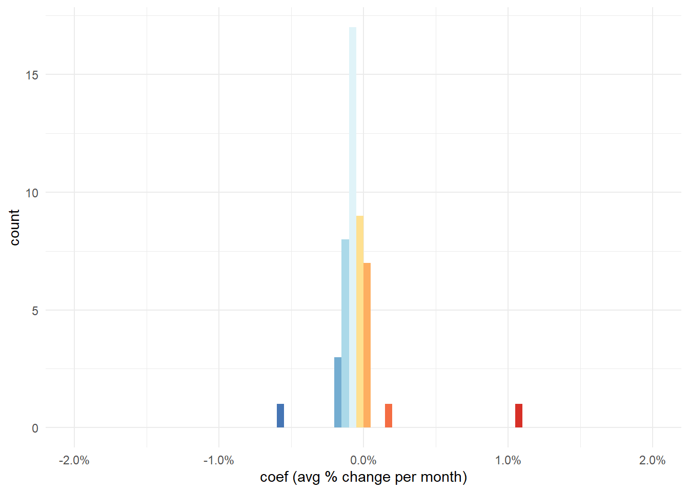
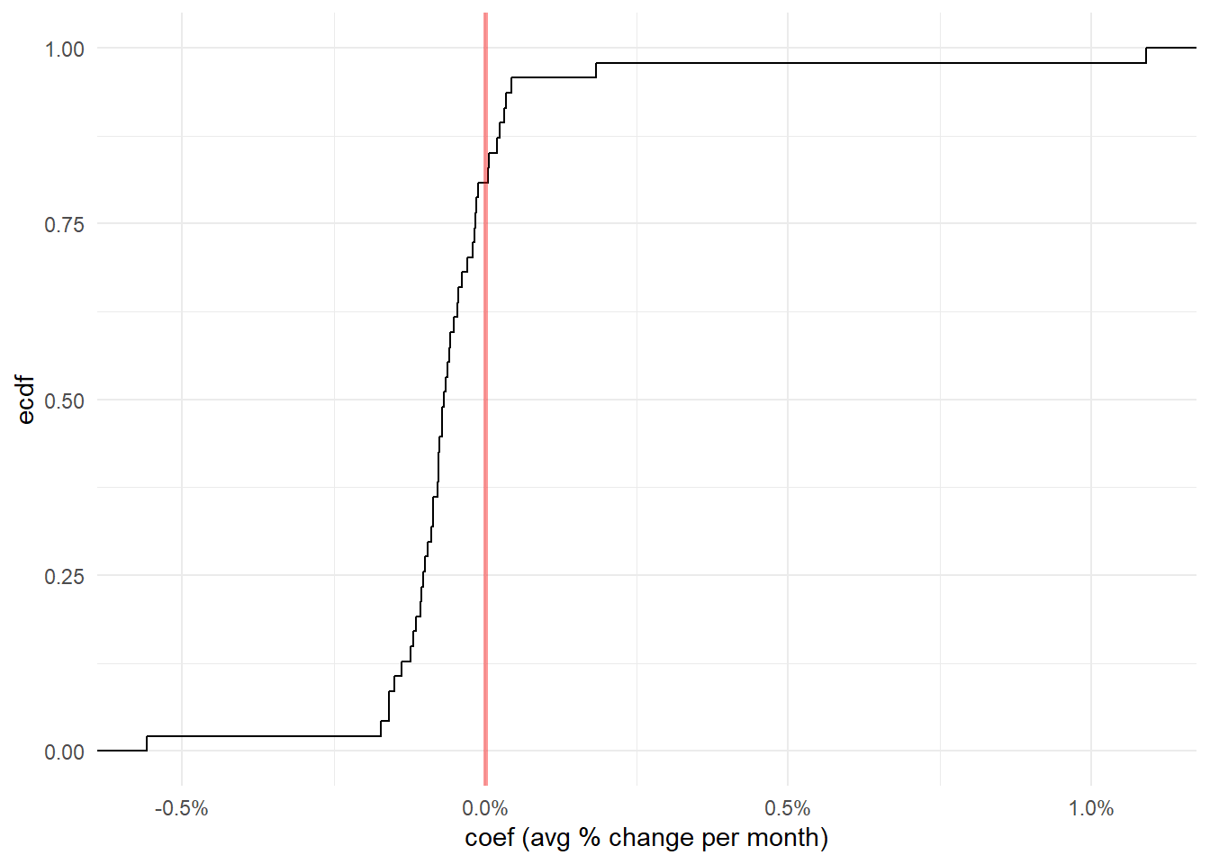
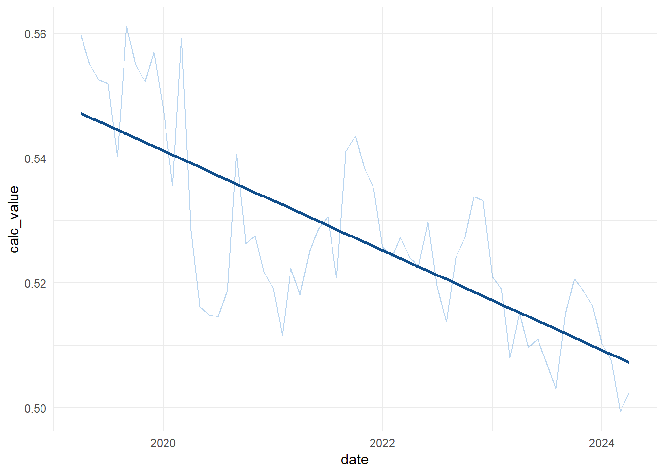
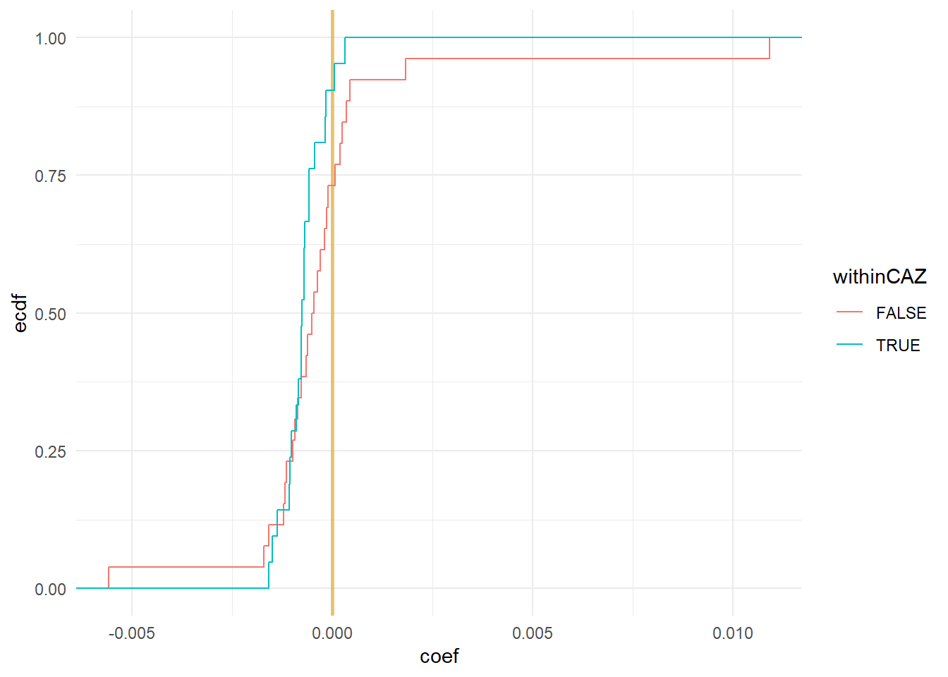
Calculating an overall trend

First let’s check the data quality for all practices and remove the NAs.

saba |>
  drop_na() |>
  summarise(n_reports = n(),
            .by = org_id) |>
  arrange(n_reports) 

# A tibble: 73 × 2
   org_id n_reports
   <chr>      <int>
 1 B83007         4
 2 B83040         7
 3 B83021        22
 4 B83006        22
 5 B82020        23
 6 B82028        23
 7 B83023        24
 8 B83027        24
 9 B83602        26
10 B83061        27
# ℹ 63 more rows

We create a vector with the ids that have more than 10 records

ids_to_include <- saba |>
  drop_na() |>
  summarise(n_reports = n(),
            .by = org_id) |>
  arrange(n_reports) |> 
  filter(n_reports>10) |> 
  pull(org_id)

Sub-setting only the relevant practices

Extracting the start month from the dataset

start_month <- min(saba$date)

Defining a function to calculate the month number of the record

diff_month <- function(start, end){
  length(seq(from=start, to=end, by='month')) - 1
}

Calculating the month difference

saba$month <- vapply(saba$date,\(x){
  diff_month(start_month,x)},numeric(1))

Subsetting the practices within the built-up area

city_practices <- Bradford_Practices[bradford_zones,] |> pull(code)

clean_data <- saba |>
  filter(org_id %in% ids_to_include,org_id %in% city_practices)

saba_processed <- clean_data |> 
  nest(data = -org_id) |> 
  mutate(lm.model = map(.x = data,
                        \(x) {
                          lm(calc_value ~ month, data = x)
                          }),
         coef = map_dbl(lm.model,\(x){coef(x)[2]})
  )

Joining trends

bradford_trends <- Bradford_Practices |>
  inner_join(
    saba_processed |>
      select(org_id,coef),
    by = c("code"="org_id"))

Mapping the trends

base_osm <- tmaptools::read_osm(bradford_trends)

tm_shape(base_osm)+
  tm_rgb()+
  tm_shape(bradford_trends |> 
  mutate(abs.size = abs(coef))
  )+
  tm_dots(col = "coef",
          midpoint = 0,
          palette = "Spectral",
          size = "abs.size",
          style = "fisher")+tm_layout(bg.color = "gray")

── tmap v3 code detected ───────────────────────────────────────────────────────

[v3->v4] `tm_dots()`: instead of `style = "fisher"`, use fill.scale =
`tm_scale_intervals()`.
ℹ Migrate the argument(s) 'style', 'midpoint', 'palette' (rename to 'values')
  to 'tm_scale_intervals(<HERE>)'
For small multiples, specify a 'tm_scale_' for each multiple, and put them in a
list: 'fill'.scale = list(<scale1>, <scale2>, ...)'
[v3->v4] `tm_dots()`: use 'fill' for the fill color of polygons/symbols
(instead of 'col'), and 'col' for the outlines (instead of 'border.col').
[cols4all] color palettes: use palettes from the R package cols4all. Run
`cols4all::c4a_gui()` to explore them. The old palette name "Spectral" is named
"brewer.spectral"
Multiple palettes called "spectral" found: "brewer.spectral", "matplotlib.spectral". The first one, "brewer.spectral", is returned.

A check of the distribution of the trends

saba_processed |> 
  filter(org_id %in% bradford_trends$code) |> 
  ggplot(aes(coef,fill = cut(coef,
                             breaks = seq(-0.02,0.02,0.0005))))+
  geom_histogram(breaks =  seq(-0.02,0.02,0.0005))+
  theme_minimal()+
  scale_x_continuous(labels = scales::percent)+
  scale_fill_brewer(palette = "RdYlBu",direction = -1)+
  labs(x = "coef (avg % change per month)")+
  theme(legend.position = "none")

saba_processed |>
  filter(org_id %in% bradford_trends$code) |> 
  ggplot(aes(coef))+
  stat_ecdf(geom = "step")+
  theme_minimal()+
  geom_vline(xintercept = 0,alpha = 0.4,col ="red",linewidth = 1)+
  scale_x_continuous(labels = scales::percent)+
  scale_fill_brewer(palette = "RdYlBu",direction = -1)+
  labs(x = "coef (avg % change per month)")+
  theme(legend.position = "none")

Calculating the overall trend

data_overall <- clean_data |>
  summarise(across(numerator:denominator,sum),
            .by = c(date, month)) |> 
  mutate(calc_value = numerator/denominator)

data_overall |> 
  ggplot(aes(date,calc_value))+
  geom_line(alpha = 0.3,
            col = "dodgerblue3")+
  geom_smooth(method = "lm",se = F,col = "dodgerblue4")+
  theme_minimal()

`geom_smooth()` using formula = 'y ~ x'

Fitting a simple linear model

lm(calc_value~month,data = data_overall) |> 
  summary()

Call:
lm(formula = calc_value ~ month, data = data_overall)

Residuals:
      Min        1Q    Median        3Q       Max 
-0.021393 -0.006513 -0.001358  0.007201  0.021795 

Coefficients:
              Estimate Std. Error t value Pr(>|t|)    
(Intercept)  5.306e-01  2.778e-03   191.0   <2e-16 ***
month       -1.134e-03  7.986e-05   -14.2   <2e-16 ***
---
Signif. codes:  0 '***' 0.001 '**' 0.01 '*' 0.05 '.' 0.1 ' ' 1

Residual standard error: 0.01098 on 59 degrees of freedom
Multiple R-squared:  0.7736,    Adjusted R-squared:  0.7698 
F-statistic: 201.6 on 1 and 59 DF,  p-value: < 2.2e-16

CAZ boundaries analysis

CAZ boundaries have been obtained from here

Reading the CAZ boundaries

CAZ_bounds <- sf::st_read("Clean_Air_Zone_Boundary.geojson") |> sf::st_transform(27700)

Reading layer `Clean_Air_Zone_Boundary' from data source 
  `C:\Users\ts18jpf\OneDrive - University of Leeds\03_PhD\00_Misc_projects\Eng-Presc-Data\Clean_Air_Zone_Boundary.geojson' 
  using driver `GeoJSON'
Simple feature collection with 1 feature and 3 fields
Geometry type: POLYGON
Dimension:     XY
Bounding box:  xmin: -1.818735 ymin: 53.7682 xmax: -1.717377 ymax: 53.84148
Geodetic CRS:  WGS 84

mapview::mapview(CAZ_bounds)

Identifying practices within the CAZ

ids_within_CAZ <- bradford_trends[CAZ_bounds,] |> pull(code)

Adding a column to identify the ones within and outside the CAZ

bradford_trends$withinCAZ <- bradford_trends$code %in% ids_within_CAZ

Exploring the distribution of coefficients (avg change per month in SABA):

bradford_trends |> 
  ggplot(aes(coef,col = withinCAZ))+
  geom_vline(xintercept = 0,col = "goldenrod",alpha = 0.6,linewidth = 1)+
  stat_ecdf()+
  theme_minimal()